Magnetometer 2
- Parent Category: Radio Astronomy
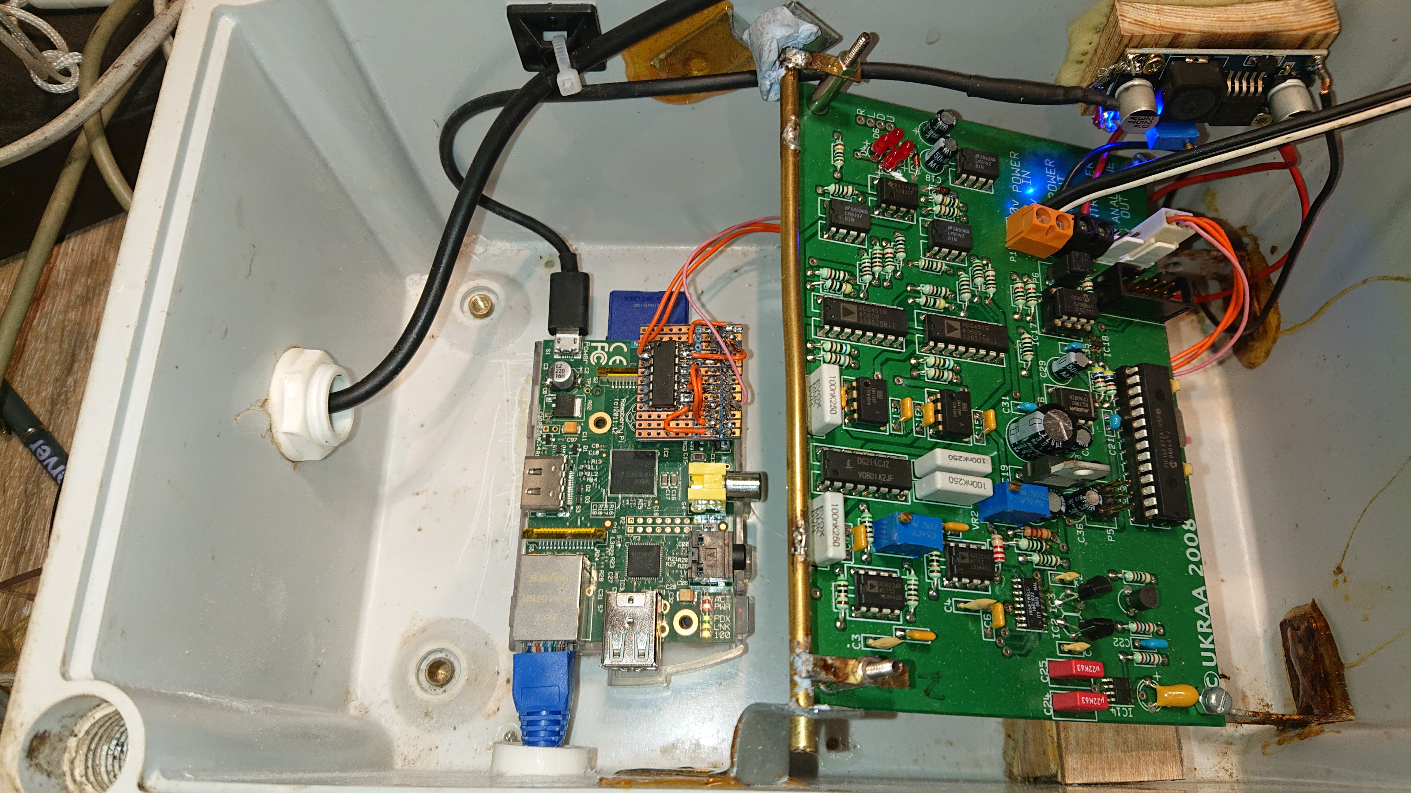
This is a prototype UKRAA Magnetometer that I built in 2008.
The original UKRAA controller has been replaced with a 2011 Raspberry Pi Model B which has been upgraded to the latest (Dec 2021) boot image with a 16GB Memory Card. The Pi is co-located with the Magnetometer in a waterproof box and fixed to a concrete plinth about half way up the garden under a hedge. Data and management is by ethernet and there is a separate power cable running to the instrument feeding 12V from a lab based power supply.
The Pi has a MCP3008 ADC (a low cost 8 channel 10bit Analogue to digital converter) piggybacked onto the IO lines. Bx and By Analogue data (0-3.3V) is fed into the Channel 0 and Channel 1 ADC GPIO inputs on the 3008.

A useful how to do it article is described here although I used a small section of Veroboard to support the 3008. Note that the Veroboard is upside down. To preserve the Pi, I used a series of female headers to link the Veroboard to the Pi GPIO pins. The only way to solder these into place is to fit the board upside down..
The magnetometer is mounted inside a Waterproof box and located on a concrete slab, about 10m away from the house and more importantly, about 30m away from the road. These are very sensitive instruments and will easily detect wagons etc on the road if located within about 10m of the road.

The Raspberry Pi is located at the bottom of the box and a small power converter to drop the feed voltage from 12V to 5V is fitted (required by the Pi). The Pi during bootup will draw about 2A of current, if there is insufficient capacity then the Pi will shut down various interface ports (including the ethernet connection) to ensure that it can operate safely. One booted and running normally, the Pi only draws about 500mA of current in this configuration.

Entry and exit for the Ethernet cable is via a 3D printed gland, well sealed with silicon sealant.

It may not be obvious, but there is a minimal amount of ferrous materials used in the box. The Pi and power supply are mounted on wooden plinths, the magnetometer pivots on a brass bar and alloy hinge points and the fine adjustment is with stainless steel screws.
Alignment is fairly simple. It needs a very firm base that has sufficient mass so that it will not move if the adjacent ground is disturbed in any way.. The board is twisted in azimuth and tilted until all 4 LEDS are extinguished. This nulls the instrument with the magnetic field at that time. Alignment is best carried out at twilight, the LEDS must be extinguished and are not easily visible when dimmed.
The Analogue output swing between 0v and 5V, with the Null set at 2.5V. However, the Pi Analogue input will only permit a maximum voltage input of 3.3V (despite use 5V as the reference voltage). It is likely that a strong magnetic storm may cause the Pi to top out if the voltage swings positive. However for most disturbances, the detectable voltage range is more than adequate.
There is no easy way of measuring the absolute strength of the earths magnetic field at a home observatory. The charts are therefore calibrated with Delta nT. Calibration is performed at the Pi, using other magnetometer data as a reference. The Python Constant corr is used in this case.
There are 3 Python3 programs used to capture and display the graphs.
The first Python program runs on the Pi reads the data every 15 seconds then integrates 10 consecutive sample to provide a smoothed output. One of the issues with an ADC is that the Analogue Output rarely matches exactly the Digital value assign. A 10bit ADC provides 1024 steps, in this case 512 steps each side of the 2.5v Null. This may seem a lot, but without integrating the data, the graph appears very noisy. Integration smooths out the noise but has secondary effect of causing a 150 second lag in the output. It is also possible that short genuine burst changes may be lost as these would be smoothed out as well. The data file contains the date, time in decimal hours, Integrated and calibrated Bx and By data and also raw Bx and By data. Always collect Raw data if possible as this can be analysed separately if required. The file format is CSV which means that is can also be easily imported into an Excel worksheet if required.
Program 1 : magreaddata.py - Python3 interpreter
import osimport datetimeimport timeimport busioimport digitalioimport boardimport adafruit_mcp3xxx.mcp3008 as MCPfrom adafruit_mcp3xxx.analog_in import AnalogIn
corr = 40 # constant to convert absolute readin to nT approx
i=0
# create the spi busspi = busio.SPI(clock=board.SCK, MISO=board.MISO, MOSI=board.MOSI)
# create the cs (chip select)cs = digitalio.DigitalInOut(board.D22)
# create the mcp objectmcp = MCP.MCP3008(spi, cs)
# create an analog input channel on pin 0 and 1chan0 = AnalogIn(mcp, MCP.P0)chan1 = AnalogIn(mcp, MCP.P1)seedx = chan0.valueseedy = chan1.valuebxarray=[seedx,seedx,seedx,seedx,seedx,seedx,seedx,seedx,seedx,seedx]byarray=[seedy,seedy,seedy,seedy,seedy,seedy,seedy,seedy,seedy,seedy]
#print (seedx,seedy)while True:
if i < 10: bxarray[i] = chan0.value byarray[i] = chan1.value else: i=0 bxarray[i] = chan0.value byarray[i] = chan1.value i=i+1# print (i,bxarray[i])# print (i,byarray[i]) chan0sm = (bxarray[0]+bxarray[1]+bxarray[2]+bxarray[3]+bxarray[4]+bxarray[5]+bxarray[6]+bxarray[7]+bxarray[8]+bxarray[9])/10 chan1sm = (byarray[0]+byarray[1]+byarray[2]+byarray[3]+byarray[4]+byarray[5]+byarray[6]+byarray[7]+byarray[8]+byarray[9])/10# print (i,chan0sm)# print (i,chan1sm)
#while True: # get date and time date = datetime.datetime.now()# print (date) filedate = (date.strftime("%Y") + date.strftime("%m") + date.strftime("%d"))# print (filedate) filepath = "/home/pi/data/" filename="mag2_" + filedate + ".csv" file = open(filepath+filename,"a") filetime = (date.strftime("%H") + date.strftime("%M") + date.strftime("%S")) filetime2 = (date.strftime("%H") + ":" + date.strftime("%M") + ":" + date.strftime("%S"))
now = datetime.datetime.now() midnight = now.replace(hour=0, minute=0, second=0, microsecond=0) seconds = (now - midnight).seconds# print(seconds) decimalhrs = seconds /3600 # print('Raw ADC0 Value: ', chan0.value)
# print('Raw ADC1 Value:', chan1.value)
file.write(filedate + "," + str(decimalhrs) + "," + str(((chan0sm-seedx))/corr) + "," + str(((chan1sm-seedy))/corr) + "," + str(chan0.value) + "," + str(chan1.value) + "\n")# print (filedate + " " + filetime +"\t" + str(chan0.value) + "\t" + str(chan1.value))
file.close()
time.sleep(15)
The other two programs run on the Server.
Program 2. This connects to the Pi using SFTP and pulls the data, copies to an array and generates the Graph. THis is fairly straightforward. no data manipulation is performed. This is called by a Cron job on the webserver, running every 5 minutes. The version shown is my local Windows PC version. It is very similar to the Unix version except for necessary changes to syntax and file locations
Program 2 : mag2dataimport.py Python 3 interpreter
#import sys#print(sys.path)import pysftpimport datetimeimport numpy as npimport matplotlib.pyplot as pltimport time
date = datetime.datetime.now()filedate = (date.strftime("%Y") + date.strftime("%m") + date.strftime("%d"))
filepath = "/home/pi/data/"filename="mag2_" + filedate + ".csv"
cnopts = pysftp.CnOpts()cnopts.hostkeys = Nonewith pysftp.Connection('192.168.0.nn', username='xxxx', password='xxxxxxxxxx') as sftp:
with sftp.cd ('data'): sftp.get(filename)
filedate = (date.strftime("%Y") + date.strftime("%m") + date.strftime("%d"))filedate2 = (date.strftime("%Y") + "-" + date.strftime("%m") + "-" + date.strftime("%d"))
filepath2 = "c:\\mag2data\\"filename2="mag2_" + filedate + ".csv"fullpath = filepath2 + filename2
filetime = (date.strftime("%H") + ":" + date.strftime("%M")) + "UTC"
mag2data = np.loadtxt(fullpath, delimiter=",")
timedata=mag2data[:,1]bxdata=mag2data[:,2]bydata=mag2data[:,3]
#draw the graphfig, ax = plt.subplots(sharex=True, figsize=(12, 6))#x=np.arange(0,24,1)
charttitle = filedate2 + " " + filetime + " -- Magnetometer 2 -- Oak Bank Observatory Willaston UK"ax.plot(timedata,bxdata, color='blue', label='Bx',lw=1)ax.plot (timedata, bydata, color='red', label = 'By',lw=1)ax.set_xlim(0,24)ax.set_ylim(-250,250)ax.set_xticks(np.arange(0,24,1))ax.set_yticks(np.arange(-250,250,50))ax.set_title(charttitle)
plt.ion()plt.xlabel("Time (Hours)")plt.ylabel("Delta nT")plt.grid(True, which='both')plt.legend()
#plt.show()image = "mag2"+filedate+".png"time.sleep(2)plt.savefig(image)plt.close('all')
The 3rd Python3 program simply copies the graph to the webserver image files folder and is called by a cron job every 5 +1 minutes.
Magnetometer2 - 7 day reports
- Parent Category: Radio Astronomy
The following graphs are in reverse chronological order commencing with a full day report from yesterday:


